Archetype0ne
Regular Member
- Messages
- 1,738
- Reaction score
- 635
- Points
- 113
- Ethnic group
- Albanian
- Y-DNA haplogroup
- L283>Y21878>Y197198
I saw a very interesting post by Nganasankhan on Anthrogenica. I asked him wether he would like to post this on Eupedia, or to get his permission to post it with credit in case he is not interested. He said he is already getting bored with genetics and had no interest joining another forum. But here are some of his posts. If any of you guys can run scripts/code, his published codes could be of great use for other populations/examples. The following post is straight copied from his thread with his permission.

The scripts in this post use the 1240K+HO dataset, which can be downloaded from here: https://reich.hms.harvard.edu/allen-...cient-dna-data.
This installs ADMIXTOOLS 2 (https://github.com/uqrmaie1/admixtools):
Code:
install.packages("devtools")
devtools::install_github("uqrmaie1/admixtools")
library("admixtools")
When I tried to install `devtools`, it failed at first because there was an error in installing the dependency `gert` of its dependency `usethis`. By running `install.packages("gert")`, I saw that I needed to run `brew install libgit2`. Even then, `admixtools` failed to install because there was an error in installing its dependency `igraph`. By googling for the error, I saw that I needed to run `brew uninstall --ignore-dependencies suite-sparse`.
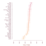
f3 as percentages with min-max scaling
This shows the amount of shared drift with Han when using Yoruba as an outgroup. The values are min-max scaled so that they are displayed on a scale where Villabruna is 0 and Nganasan is 100.
Code:
$ Printf% s \\ n Bashkir Besermyan Chuvash Enets Estonia_N_CombCeramic.SG Estonian.DG Finnish Finnish.DG Hungarian.DG Italy_North_Villabruna_HG Karelian Mansi Mari.SG Mordovian Nganasan Norway_Viking_o1.SG Russia_Bolshoy Russia_Chalmny_Varre Russia_Chalmny_Varre Russia_EHG Russia_MLBA_Krasnoyarsk_o Russia_Shamanka_Eneolithic.SG Saami.DG Selkup Tatar_Mishar Tatar_Siberian_Zabolotniye Todzin Tofalar Udmurt> pops
$ R -e 'library(tidyverse);library(admixtools);f3=f3("path/to/v44.3_HO_public","Yoruba","Han",readLines("pops"))%>%arrange(est);est=f3$est-min(f3$est);est=est/max(est);cat(paste(round(100*est),f3$pop3),sep="\n")'
[...]
0 Italy_North_Villabruna_HG
2 Hungarian.DG
6 Estonian.DG
12 Finnish.DG
12 Mordovian
13 Finnish
13 Russia_EHG
14 Karelian
20 Tatar_Mishar
26 Besermyan
27 Chuvash
28 Mari.SG
29 Russia_Chalmny_Varre
30 Udmurt
33 Saami.DG
37 Russia_MLBA_Krasnoyarsk_o
38 Bashkir
40 Norway_Viking_o1.SG
54 Russia_Bolshoy
55 Tatar_Siberian_Zabolotniye
57 Mansi
70 Selkup
80 Enets
90 Tofalar
94 hours
99 Russia_Shamanka_Eneolithic.SG
100 Nganasan
If you get a low number of SNPs that remain after filtering, try to remove samples with a low SNP count. For example in a run before the run shown above, my SNP count was 12245. I ran a command like this to find samples with a low SNP count:
Code:
$ awk -F\\t 'NR==FNR{a[$0];next}$8 in a{print$15,$8,$2}' pops path/to/v44.3_HO_public.anno|sort -n|head -n8
30001 Estonia_N_CombCeramic.SG MA974.SG
58972 Estonia_N_CombCeramic.SG MA975.SG
201719 Russia_Chalmny_Varre CHV002.A0101
205900 Norway_Viking_o1.SG VK518.SG
218757 Russia_Shamanka_Eneolithic.SG DA251.SG
287462 Russia_Bolshoy BOO002.A0101
289954 Russia_EHG UzOO77
300800 Russia_Shamanka_Eneolithic.SG DA250.SG
After I removed Estonia_N_CombCeramic.SG, my SNP count increased to 73054.
f3 as a heatmap
This applies min-max scaling to f3 values and displays the scaled values as percentages:
Code:
library(tidyverse)
library(admixtools)
library(pheatmap)
library(colorspace)
minmax=function(x)(x-min(x,na.rm=T))/(max(x,na.rm=T)-min(x,na.rm=T))
p1="Yoruba.DG"
p2=c("Nganasan","Russia_HG_Karelia","Norway_N_HG.SG","Turkey_N","Russia_HG_Tyumen","Han","Estonia_CordedWare","Russia_Bolshoy","Luxembourg_Loschbour","Russia_Samara_EBA_Yamnaya","Georgia_Kotias.SG")
p3=c("Nganasan","Estonian.DG","Selkup","Hungarian.DG","Karelian","Mansi","Udmurt","Mordovian","Saami.DG","Besermyan","Finnish","Finland_Levanluhta","Tofalar","Russia_MLBA_Krasnoyarsk_o","Russia_Bolshoy","Enets","Russia_Chalmny_Varre","Norwegian")
f3=f3("path/to/v44.3_HO_public",p1,p2,p3)
t=f3%>%select(pop2,pop3,est)%>%pivot_wider(names_from=pop2,values_from=est)%>%data.frame(row.names=1)
# don't show the f3 values of populations with themselves in order to not stretch the color scale
makena=names(which(sapply(rownames(t),function(x)any(names(t)==x))))
lapply(makena,function(x)t[x,x]<<-NA)
range=apply(t,2,function(x)paste(sub("^0","",sprintf("%.3f",range(x,na.rm=T))),collapse="-"))
names(t)=paste0(names(t)," (",range,")")
t=minmax(t) # use the same scale for the whole table
# t=apply(t,2,function(x)minmax(x)) # scale each column individually
pheatmap (
t*100,filename="a.png",
# cluster_cols=F,cluster_rows=F,
treeheight_row=70,treeheight_col=70,
legend=F,cellwidth=16,cellheight=16,fontsize=8,border_color=NA,
display_numbers=T,number_format="%.0f",fontsize_number=7,number_color="black",
colorRampPalette(colorspace::hex(HSV(c(210,170,120,60,40,20,0),.5,1)))(256)
)
Here min-max scaling was applied to the whole table on the left side and to each column individually on the right side:

The script below displays the original f3 values without scaling. It also demonstrates how `vegan::reorder.hclust` can be used to reorder the branches of the heatmap.
Code:
library(tidyverse)
library(admixtools)
library(pheatmap)
library(colorspace) # for hex
library(vegan) # for reorder.hclust
p1="Yoruba.DG"
p2=c("Nganasan","Russia_HG_Karelia","Norway_N_HG.SG","Turkey_N","Russia_HG_Tyumen","Han","Estonia_CordedWare","Russia_Bolshoy","Luxembourg_Loschbour","Russia_Samara_EBA_Yamnaya","Georgia_Kotias.SG","Finnish","Finland_Levanluhta","Russia_Shamanka_Eneolithic.SG")
f3=f3("path/to/v44.3_HO_public",p1,p2,p2)
t=f3%>%select(pop2,pop3,est)%>%pivot_wider(names_from=pop2,values_from=est)%>%data.frame(row.names=1)
diag(t)=NA # don't show the f3 values of populations with themselves in order to not stretch the color scale
pheatmap (
t,filename="a.png",
clustering_callback=function(...){reorder(hclust(dist(t)),wts=t[,"Han"]-t[,"Turkey_N"])},
display_numbers=apply(t,1,function(x)sub("^0","",sprintf("%.3f",x))),
legend=F,border_color=NA,cellwidth=16,cellheight=16,fontsize=8,fontsize_number=7,number_color="black",
# breaks=seq(.160,.190,.03/256), # use fixed limits for color scale
colorRampPalette(hex(HSV(c(210,170,120,60,40,20,0),.5,1)))(256)
)
Result:

f3-outgroup nMonte
This saves an f3 table as a CSV file so it can be used with Vahaduo or nMonte. It uses a shell wrapper for my simplified version of nMonte3.R.
Code:
$ printf% s \\ n Estonia_CordedWare Finland_Levanluhta Finnish Georgia_Kotias.SG Han Luxembourg_Loschbour Nganasan Norway_N_HG.SG Russia_Bolshoy Russia_HG_Karelia Russia_HG_Tyumen Russia_Samara_EBA_Yamnaya Turkey_Shamanka_EBA_Yamnaya Turkey_Shamanka_EBA
$ R -e 'library(tidyverse);library(admixtools);pops=readLines("pops");f3=f3("path/to/v44.3_HO_public","Yoruba.DG",pops,pops);f3%>%select(pop2,pop3,est)%>%pivot_wider(names_from=pop3,values_from=est)%>%mutate(across(where(is.double),round,6))%>%write_csv("f3")'
$ cat f3
pop2,Estonia_CordedWare,Finland_Levanluhta,Finnish,Georgia_Kotias.SG,Han,Luxembourg_Loschbour,Nganasan,Norway_N_HG.SG,Russia_Bolshoy,Russia_HG_Karelia,Russia_HG_Tyumen,Russia_Samara_EBA_Yamnaya,Russia_Shamanka_Eneolithic.SG,Turkey_N
Estonia_CordedWare,0.189574,0.048826,0.050368,0.046842,0.040376,0.05185,0.042084,0.049919,0.04784,0.050933,0.047266,0.051533,0.040938,0.049494
Finland_Levanluhta, 0.048826,0.148686,0.051402,0.045953,0.045448,0.052605,0.048901,0.053542,0.052522,0.053938,0.054203,0.051491,0.046715,0.048399
Finnish,0.050368,0.051402,0.052422,0.047057,0.042304,0.053757,0.04443,0.052616,0.048967,0.053264,0.049454,0.050761,0.04272,0.0495
Georgia_Kotias.SG,0.046842,0.045953,0.047057,0.185421,0.0394,0.045323,0.041384,0.046218,0.044534,0.047698,0.044243,0.048927,0.040304,0.046263
Han, 0.040376,0.045448,0.042304,0.0394,0.061217,0.040942,0.057035,0.041632,0.049274,0.043826,0.044467,0.040925,0.057394,0.038767
Luxembourg_Loschbour,0.05185,0.052605,0.053757,0.045323,0.040942,0.188232,0.043033,0.062498,0.050054,0.057409,0.049533,0.051483,0.04226,0.049539
Nganasan,0.042084,0.048901,0.04443,0.041384,0.057035,0.043033,0.070154,0.04448,0.054056,0.047517,0.047917,0.043077,0.059516,0.039822
Norway_N_HG.SG,0.049919,0.053542,0.052616,0.046218,0.041632,0.062498,0.04448,0.189739,0.053043,0.062429,0.053055,0.052822,0.043558,0.048115
Russia_Bolshoy, 0.04784,0.052522,0.048967,0.044534,0.049274,0.050054,0.054056,0.053043,0.063846,0.057001,0.054654,0.049657,0.051358,0.04458
Russia_HG_Karelia,0.050933,0.053938,0.053264,0.047698,0.043826,0.057409,0.047517,0.062429,0.057001,0.170124,0.062403,0.055766,0.046348,0.048079
Russia_HG_Tyumen,0.047266,0.054203,0.049454,0.044243,0.044467,0.049533,0.047917,0.053055,0.054654,0.062403,0.18867,0.054148,0.046497,0.043883
Russia_Samara_EBA_Yamnaya, 0.051533,0.051491,0.050761,0.048927,0.040925,0.051483,0.043077,0.052822,0.049657,0.0557660,0.0.05414,05414
Russia_Shamanka_Eneolithic.SG,0.040938,0.046715,0.04272,0.040304,0.057394,0.04226,0.059516,0.043558,0.051358,0.046348,0.046497,0.041908,0.064461,0.039068
Turkey_N,0.049494,0.048399,0.0495,0.046263,0.038767,0.049539,0.039822,0.048115,0.04458,0.048079,0.043883,0.047615,0.039068,0.055858
$ nm()(grep -v ^, "$1">/tmp/nm1;grep -v ^, "$2">/tmp/nm2;Rscript -e 'source("~/bin/nmon.R");a=as.numeric(commandArgs(T));getMonte("/tmp/nm1","/tmp/nm2",Nbatch=a[1],Ncycles=a[2],pen=a[3])' "${3-500}" "${4-1000}" "${5-.001}")
$ nm <(sed 1d f3|grep -v Finnish) <(sed 1d f3|grep Finnish)
Target: Finnish (d=.0028)
45.2 Russia_Samara_EBA_Yamnaya
35.6 Turkey_N
5.0 Russia_Bolshoy
3.4 Nganasan
3.0 Han
2.6 Luxembourg_Loschbour
1.4 Finland_Levanluhta
1.4 Norway_N_HG.SG
1.2 Russia_Shamanka_Eneolithic.SG
0.8 Russia_HG_Karelia
0.4 Estonia_CordedWare
$ cat ~/bin/nmon.R
getMonte=function(datafile,targetfile,Nbatch=500,Ncycles=1000,pen=0){
do_algorithm=function(selection,targ){
mySel = as.matrix (selection, rownames.force = NA)
myTg=as.matrix(targ,rownames.force=NA)
dif2targ=sweep(mySel,2,myTg,"-")
Ndata = nrow (dif2targ)
kcol=ncol(dif2targ)
rowLabels=rownames(dif2targ)
matPop=matrix(NA_integer_,Nbatch,1,byrow=T)
dumPop=matrix(NA_integer_,Nbatch,1,byrow=T)
matAdmix=matrix(NA_real_,Nbatch,kcol,byrow=T)
dumAdmix=matrix(NA_real_,Nbatch,kcol,byrow=T)
matPop = sample (1: Data, Nbatch, replace = T)
matAdmix=dif2targ[matPop,]
colM1 = colMeans (matAdmix)
eval1=(1+pen)*sum(colM1^2)
for(c in 1:Ncycles){
dumPop=sample(1:Ndata,Nbatch,replace=T)
dumAdmix=dif2targ[dumPop,]
for(b in 1:Nbatch){
store=matAdmix[b,]
matAdmix[b,]=dumAdmix[b,]
colM2 = colMeans (matAdmix)
eval2=sum(colM2^2)+pen*sum(matAdmix[b,]^2)
if(eval2<=eval1){
matPop=dumPop
colM1=colM2
eval1=eval2
}else{matAdmix[b,]=store}
}
}
fitted = t (colMeans (matAdmix) + myTg [1,])
popl=unlist(lapply(strsplit(rowLabels[matPop],";"),function(x)x[1]))
populations=factor(popl)
return(list("estimated"=fitted,"pops"=populations))
}
source=read.csv(datafile,header=F,row.names=1)
target=read.csv(targetfile,header=F,row.names=1)
for(i in 1:nrow(target)){
row=target[i,]
result=do_algorithm(source,row)
if(i>=2)cat("\n")
dist=sqrt(sum((result$estimated-row)^2))
cat(paste0("Target: ",row.names(row)," (d=",sub("^0","",sprintf("%.4f",dist)),")\n"))
tb=table(result$pops)
tb=sort(tb,decreasing=T)
tb=as.matrix(100*tb/Nbatch)
cat(paste(sprintf("%.1f",tb),row.names(tb)),sep="\n")
}
}
qpGraph with predefined node list
Code:
t=read.table(text="R Yoruba.DG
R A
TO THE
A AA
OE
O ONLY
AND I
E L1
I WH
I EH
AA EH
EH EH2
EH EH1
EH AAA
AA AAA
WH CCE
WH Italy_North_Villabruna_HG
CH YM
CH CH1
CH ON
EH1 YM
EH1 EH0
AAA AAN
CH1 EH0
CH1 Georgia_Kotias.SG
L1 Turkey_N_published
L1 LB
L1 YM1
L1 CW
EH2 LB
EH2 CWC
YM YM1
YM CW
EH0 Russia_HG_Karelia
AAN Nganasan
TO CCA
LB Germany_EN_LBK
LB CCW
YM1 Russia_Samara_EBA_Yamnaya
CW CCW
CW Estonia_CordedWare
CCW CWC
CWC CCE
CCE CCA
CCA Finnish.DG")
pop=c("Finnish.DG","Estonia_CordedWare","Germany_EN_LBK","Italy_North_Villabruna_HG","Nganasan","Russia_HG_Karelia","Russia_Samara_EBA_Yamnaya","Turkey_N_published","Yoruba.DG","Georgia_Kotias.SG")
f2=f2_from_geno("path/to/v44.3_HO_public",pops=pop)
gr=qpgraph(f2,t)
plot_graph(gr$edges)
ggsave("a.png",width=9,height=9)
system("mogrify -trim -border 64 -bordercolor white a.png")
plotly_graph(gr$edges) # view Plotly graph in browser
In order to generate a black-and-white graph, run `write_dot(gr$edges)` and paste the output here: http://viz-js.com.

qpAdm popdrop table as a stacked bar chart
The `popdrop` table contains alternative models for each non-empty subset of the left populations. The script below selects all models from the `popdrop` table with zero negative weights (where the value of the `feasible` column is not false) and with at least two left populations (where `f4rank` is not 0). It then plots the models sorted by their p score.
In qpAdm, the number of right populations needs to be greater than or equal to the number of left populations. Otherwise you'll get an error like this: `Error in qpadm_weights(f4_est, qinv, rnk = length(left) - 2, fudge = fudge: Mat::cols(): indices out of bounds or incorrectly used`.
I'm still afraid of qpAdm because I have no idea how to choose the outgroups, but I just selected a subset of the outgroups that were used in the paper titled "The Genomic History of Southeastern Europe": https://anthrogenica.com/showthread....pains-of-qpAdm. When the genetic distance between the right populations to left populations is high like in my model, the p values also tend to be higher.
Code:
library(admixtools)
library(tidyverse)
library(reshape2) # for melt
library(colorspace) # for hex
library(cowplot) # for plot_grid
left=c("Turkey_Boncuklu_N.SG","Estonia_CordedWare.SG","Latvia_HG","Russia_HG_Karelia","Finland_Levanluhta","Nganasan")
right=c("Ethiopia_4500BP_published.SG","Mbuti.DG","Russia_Ust_Ishim_HG_published.DG","Karitiana.DG","Papuan.DG","ONG.SG")
target="Mari.SG"
qp=qpadm("path/to/v44.3_HO_public",left,right,target)
t=qp$popdrop%>%filter(feasible==T&f4rank!=0)%>%arrange(desc(p))%>%select(1,4,5,7:last_col(5))
t2=melt(t[-c(2,3)],id.vars="pat") # this uses `melt` because `pivot_longer` doesn't preserve the order of columns
lab=sub("e-0","e-",sub("^0","",sprintf(ifelse(t$p<.001,"%.0e","%.3f"),t$p)))
lab=paste0(lab," (",ifelse(t$chisq<10,sub("^0","",sprintf("%.1f",t$chisq)),round(t$chisq)),")")
subtit=str_wrap(paste("Right:",paste(sort(right),collapse=", ")),width=58)
p=ggplot(t2,aes(x=fct_rev(factor(pat,level=t$pat)),y=value,fill=variable))+
geom_bar(stat="identity",width=1,position=position_fill(reverse=T))+
geom_text(aes(label=round(100*value)),position=position_stack(vjust=.5,reverse=T),size=3.5)+
ggtitle(paste("Target:",target),subtitle=subtit)+
coord_flip()+
scale_x_discrete(expand=c(0,0),labels=rev(lab))+
scale_y_discrete(expand=c(0,0))+ # remove gray margins on the left and right side of the plot
scale_fill_manual("legend",values=hex(HSV(c(30,60,180,210,270,330),.5,1)))+ # use manual colors
# scale_fill_manual(values=colorspace::hex(HSV(head(seq(0,360,length.out=1+ncol(t)-3),-1),.5,1)))+ # use automatic colors
guides(fill=guide_legend(ncol=2,byrow=F))+
theme(
axis.text.x=element_blank(),
axis.text.y=element_text(size=11),
axis.text=element_text(color="black"),
axis.ticks=element_blank(),
axis.title=element_blank(),
legend.direction="horizontal",
legend.key=element_rect(fill=NA), # remove gray border around color squares
legend.margin=margin(-4,0,1,0),
legend.text=element_text(size=11),
legend.title=element_blank(),
plot.subtitle=element_text(size=12),
plot.title=element_text(size=16)
)
ggdraw(p)
hei=c(.5+.2*(str_count(subtit,"\n")+1)+.25*nrow(t),.1+.23*ceiling(length(unique(t2[!is.na(t2$value),2]))/2))
ggdraw(plot_grid(p+theme(legend.position="none"),get_legend(p),ncol=1,rel_heights=hei))
ggsave("a.png",width=5.5,height=sum(hei))
In the image below, the number in parenthes after the p-value is chi-squared. Models with a large number of left populations tend to get a low chi-squared relative to the p-value. Models with only two left populations tend to get a high chi-squared relative to the p-value.

Print qpAdm popdrop table as plain text
Code:
library(admixtools)
library(tidyverse)
left=c("Turkey_Boncuklu_N.SG","Russia_Samara_EBA_Yamnaya","Latvia_HG","Russia_HG_Karelia","Nganasan","Finland_Levanluhta","Russia_Bolshoy")
right=c("Russia_Ust_Ishim_HG_published.DG","Russia_HG_Tyumen","Belgium_UP_GoyetQ116_1_published_all","Russia_Kostenki14","Iran_Wezmeh_N.SG","Georgia_Kotias.SG","Turkey_Epipaleolithic","China_YR_LN")
target="Finnish"
qp=qpadm("path/to/v44.3_HO_public",left,right,target)
t=qp$popdrop%>%filter(feasible==T&f4rank!=0)%>%arrange(desc(p))
p=apply(t%>%select(7:last_col(5)),1,function(x){y=round(100*sort(na.omit(x),decreasing=T));paste(paste0(y,"% ",names") ),collapse=" + ")})
),collapse=" + ")})
paste0(sub("^0","",sprintf(ifelse(t$p<.001,"%.0e","%.3f"),t$p)),": ",p)%>%cat(sep="\n")
Output:
.630: 45% Russia_Samara_EBA_Yamnaya + 28% Turkey_Boncuklu_N.SG + 15% Latvia_HG + 11% Nganasan
.335: 41% Finland_Levanluhta + 35% Russia_Samara_EBA_Yamnaya + 24% Turkey_Boncuklu_N %vanaya
Russia_Samnaya_25_Boncuklu_N% % Turkey_Boncuklu_N.SG + 2% Nganasan
.011: 38% Russia_Samara_EBA_Yamnaya + 34% Turkey_Boncuklu_N.SG + 23% Russia_Bolshoy + 5% Latvia_HG
.010: 46% Russia_Samara_EBA_Yamnaya + 34%
Turkey_NGoncuklukluk : 42% Russia_Samara_EBA_Yamnaya + 35% Turkey_Boncuklu_N.SG + 24% Russia_Bolshoy
.004: 49% Russia_Samara_EBA_Yamnaya + 33% Turkey_Boncuklu_N.SG + 11% Nganasan + 7% Russia_HG_Karelia
.002: 58% Russia_Samara_EBA_Yamnaya + 31% Turkey_Boncuklu_N.SG + 12% Nganasan
7e-11: 50% Finland_Levanluhta + 35% Turkey_Boncuklu_N.SG + 16% Russia_HG_Karelia
5e-12: 59% Finland_Levan_Bluhta + Latvia.SG
7e-13: 52% Turkey_Boncuklu_N.SG + 39% Russia_HG_Karelia + Nganasan 9%
4e-13: 69% Finland_Levanluhta + Turkey_Boncuklu_N.SG 31%
2e-14: 52% Turkey_Boncuklu_N.SG + 27% Russia_HG_Karelia + Russia_Bolshoy 21%
1e-19 : 46% Turkey_Boncuklu_N.SG + 28% Russia_Bolshoy + 26% Latvia_HG
1e-23: 71% Finland_Levanluhta + 29% Russia_Samara_EBA_Yamnaya
4e-24: 54% Turkey_Boncuklu_N.SG + 46% Russia_HG_Karelia% Turkey 2N
-26_G Latvia_HG + 12% Nganasan
7e-27: 63% Turkey_Boncuklu_N.SG + 37% Russia_Bolshoy
8e-36: 55% Russia_Samara_EBA_Yamnaya + 36% Turkey_Boncuklu_N.SG + 9% Latvia_HG
6e-38: 63% Russia_Samara_EBA_Yamnaya + 37% Turkey_NBoncuk
5% .SG + Nganasan 15%
4e-53: 56% Turkey_Boncuklu_N.SG + Latvia_HG 44%
7e-61: 85% Russia_Samara_EBA_Yamnaya + 10% Nganasan + Latvia_HG 5%
4e-62: 90% Russia_Samara_EBA_Yamnaya + Nganasan 10%
3e-76: 98 % Russia_HG_Karelia + 2% Nganasan
5e-78: 88% Russia_Samara_EBA_Yamnaya + 12% Russia_Bolshoy
2e-116: 91% Latvia_HG + 9% Nganasan
1e-128: 92% Latvia_HG + 8% Russia_Bolshoy
plot_map
The `plot_map` function uses Plotly to generate an interactive map for entries from an anno file. You can see the code of the function by running `plot_map`.
Code:
library(admixtools)
library(tidyverse)
t=as.data.frame(read_tsv(gsub("\u00a0"," ",read_file("path/to/v44.3_HO_public.anno")))) # remove non-breaking spaces so `as.numeric` won't fail
t=t[,c(8,11,12,6)] # group, latitude, longitude, years BP
t=t[!grepl("\\.REF|rel\\.|fail\\.|Ignore_|_dup|_contam|_lc|_father|_mother|_son|_daughter|_brother|_sister|_sibling|_twin|Neanderthal|Denisova|Vindija_light|Gorilla|Macaque|Marmoset|Orangutang|Primate_Chimp|hg19ref|_o|_outlier",t[,1]),]
t=t[t[,2]!=".."&t[,3]!=".."&t[,2]!="-"&t[,3]!="-",] # remove lines with missing lat or long field (can be `..` or `-`)
t[t[,4]==0,4]=1 # change years BP 0 to 1 because entries with years BP 0 are not plotted when using a log scale (which is the default option)
a=aggregate(apply(t[,-1],2,as.numeric),list(t[,1]),mean)
a[,5]=a[,1]
names(a)=c("iid","lat","lon","yearsbp","group")
admixtools:lot_map(a)

A second option is to first run this in a shell:
Code:
$ igno()(grep -Ev '\.REF|rel\.|fail\.|Ignore_|_dup|_contam|_lc|_father|_mother|_son|_daughter|_brother|_sister|_sibling|_twin|Neanderthal|Denisova|Vindija_light|Gorilla|Macaque|Marmoset|Orangutang|Primate_Chimp|hg19ref')
$ tav()(awk '{n[$1]++;for(i=2;i<=NF;i++){a[$1]+=$i}}END{for(i in a){o=i;for(j=2;j<=NF;j++)o=o FS sprintf("%f",a[j]/n);print o}}' "FS=${1-$'\t'}")
$ awk -F\\t 'NR>1&&$11!=".."&&$11!="-"{print$8,$11,$12,$6}' path/to/v44.3_HO_public.anno|igno|grep -v _o|tav \ >map
$ head -n2 map
Ireland_EBA.SG 55.292132 -6.191685 3765.333333
Germany_EN_LBK 49.674249 9.582716 7066.370370
Then run this in R:
Code:
t=read.table("map");t[t[,4]==0,4]=1;t[,5]=t[,1];names(t)=c("iid","lat","lon","yearsbp","group");plot_map(t)'
A third option is to use Plotly directly:
Code:
library(plotly)
a=read.table("map")
label=ifelse(a[,4]==0,a[,1],paste0(a[,1],"\u00a0",round(a[,4])))
pl=plot_ly(a,type="scattermapbox",mode="markers",x=a[,3],y=a[,2],text=a[,1],hovertext=label,hoverinfo="text",marker=list(size=8,color=log10(a[,4]),colorscale="Portland",colorbar=list(thickness=15,outlinewidth=0)))
plotly::layout(pl,mapbox=list(style="stamen-terrain"),margin=list(t=0,r=0,b=0,l=0,pad=0))
In order to display the names of populations in addition to dots, you can use `mode="markers+text"`. It is currently only supported by the mapbox map styles which require a free access token: https://community.plotly.com/t/scatt...-as-text/35065. The `satellite-streets` style also includes the names of cities but `satellite` doesn't.
Code:
library(plotly)
a=read.table("map")
label=ifelse(a[,4]==0,a[,1],paste0(a[,1],"\u00a0",round(a[,4])))
pl=plot_ly(a,type="scattermapbox",mode="markers+text",x=a[,3],y=a[,2],text=label,textfont=list(color="white"),textposition="top",marker=list(color=log10(a[,4]),size=8,colorscale="Jet"))
plotly::layout(pl,mapbox=list(style="satellite-streets",accesstoken="youraccesstoken"),margin=list(t=0,r=0,b=0,l=0,pad=0))

FST or f2 heatmap
The default clustering method used by `pheatmap` is equivalent to `hclust(dist(t))`. Here the input is already a distance matrix, so you can use this instead: `clustering_callback=function(...)hclust(as.dist(t ))`.
Code:
library(admixtools)
library(pheatmap)
library(vegan) # for reorder.hclust
library(colorspace) # for hex
pop=unlist(strsplit("Besermyan Enets Estonian Finnish Hungarian Karelian Mansi Mordovian Nganasan Saami.DG Selkup Udmurt"," "))
f=fst("path/to/v44.3_HO_public",pop)
# f=f2("path/to/v44.3_HO_public",pop)
# convert FST or f2 pairs to square matrix
df=as.data.frame(f[,-4])
df2=rbind(df,setNames(df[,c(2,1,3)],names(df)))
t=xtabs(df2[,3]~df2[,1]+df2[,2])
weights=t["Hungarian",]-t["Nganasan",]
# weights=rowMeans(t) # sort by average distance to other populations
pheatmap (
1000*t,filename="a.png",
clustering_callback=function(...)reorder(hclust(as.dist(t)),weights),
# clustering_callback=function(...)hclust(as.dist(t)),
legend=F,border_color=NA,cellwidth=18,cellheight=18,
treeheight_row=80,treeheight_col=80,
display_numbers=T,number_format="%.0f",number_color="black",
colorRampPalette(hex(HSV(c(210,210,130,60,40,20,0),c(0,.5,.5,.5,.5,.5,.5),1)))(256)
)
Here the FST values are multiplied by 1,000 and not by 10,000 as usual:

The scripts in this post use the 1240K+HO dataset, which can be downloaded from here: https://reich.hms.harvard.edu/allen-...cient-dna-data.
This installs ADMIXTOOLS 2 (https://github.com/uqrmaie1/admixtools):
Code:
install.packages("devtools")
devtools::install_github("uqrmaie1/admixtools")
library("admixtools")
When I tried to install `devtools`, it failed at first because there was an error in installing the dependency `gert` of its dependency `usethis`. By running `install.packages("gert")`, I saw that I needed to run `brew install libgit2`. Even then, `admixtools` failed to install because there was an error in installing its dependency `igraph`. By googling for the error, I saw that I needed to run `brew uninstall --ignore-dependencies suite-sparse`.
f3 as percentages with min-max scaling
This shows the amount of shared drift with Han when using Yoruba as an outgroup. The values are min-max scaled so that they are displayed on a scale where Villabruna is 0 and Nganasan is 100.
Code:
$ Printf% s \\ n Bashkir Besermyan Chuvash Enets Estonia_N_CombCeramic.SG Estonian.DG Finnish Finnish.DG Hungarian.DG Italy_North_Villabruna_HG Karelian Mansi Mari.SG Mordovian Nganasan Norway_Viking_o1.SG Russia_Bolshoy Russia_Chalmny_Varre Russia_Chalmny_Varre Russia_EHG Russia_MLBA_Krasnoyarsk_o Russia_Shamanka_Eneolithic.SG Saami.DG Selkup Tatar_Mishar Tatar_Siberian_Zabolotniye Todzin Tofalar Udmurt> pops
$ R -e 'library(tidyverse);library(admixtools);f3=f3("path/to/v44.3_HO_public","Yoruba","Han",readLines("pops"))%>%arrange(est);est=f3$est-min(f3$est);est=est/max(est);cat(paste(round(100*est),f3$pop3),sep="\n")'
[...]
0 Italy_North_Villabruna_HG
2 Hungarian.DG
6 Estonian.DG
12 Finnish.DG
12 Mordovian
13 Finnish
13 Russia_EHG
14 Karelian
20 Tatar_Mishar
26 Besermyan
27 Chuvash
28 Mari.SG
29 Russia_Chalmny_Varre
30 Udmurt
33 Saami.DG
37 Russia_MLBA_Krasnoyarsk_o
38 Bashkir
40 Norway_Viking_o1.SG
54 Russia_Bolshoy
55 Tatar_Siberian_Zabolotniye
57 Mansi
70 Selkup
80 Enets
90 Tofalar
94 hours
99 Russia_Shamanka_Eneolithic.SG
100 Nganasan
If you get a low number of SNPs that remain after filtering, try to remove samples with a low SNP count. For example in a run before the run shown above, my SNP count was 12245. I ran a command like this to find samples with a low SNP count:
Code:
$ awk -F\\t 'NR==FNR{a[$0];next}$8 in a{print$15,$8,$2}' pops path/to/v44.3_HO_public.anno|sort -n|head -n8
30001 Estonia_N_CombCeramic.SG MA974.SG
58972 Estonia_N_CombCeramic.SG MA975.SG
201719 Russia_Chalmny_Varre CHV002.A0101
205900 Norway_Viking_o1.SG VK518.SG
218757 Russia_Shamanka_Eneolithic.SG DA251.SG
287462 Russia_Bolshoy BOO002.A0101
289954 Russia_EHG UzOO77
300800 Russia_Shamanka_Eneolithic.SG DA250.SG
After I removed Estonia_N_CombCeramic.SG, my SNP count increased to 73054.
f3 as a heatmap
This applies min-max scaling to f3 values and displays the scaled values as percentages:
Code:
library(tidyverse)
library(admixtools)
library(pheatmap)
library(colorspace)
minmax=function(x)(x-min(x,na.rm=T))/(max(x,na.rm=T)-min(x,na.rm=T))
p1="Yoruba.DG"
p2=c("Nganasan","Russia_HG_Karelia","Norway_N_HG.SG","Turkey_N","Russia_HG_Tyumen","Han","Estonia_CordedWare","Russia_Bolshoy","Luxembourg_Loschbour","Russia_Samara_EBA_Yamnaya","Georgia_Kotias.SG")
p3=c("Nganasan","Estonian.DG","Selkup","Hungarian.DG","Karelian","Mansi","Udmurt","Mordovian","Saami.DG","Besermyan","Finnish","Finland_Levanluhta","Tofalar","Russia_MLBA_Krasnoyarsk_o","Russia_Bolshoy","Enets","Russia_Chalmny_Varre","Norwegian")
f3=f3("path/to/v44.3_HO_public",p1,p2,p3)
t=f3%>%select(pop2,pop3,est)%>%pivot_wider(names_from=pop2,values_from=est)%>%data.frame(row.names=1)
# don't show the f3 values of populations with themselves in order to not stretch the color scale
makena=names(which(sapply(rownames(t),function(x)any(names(t)==x))))
lapply(makena,function(x)t[x,x]<<-NA)
range=apply(t,2,function(x)paste(sub("^0","",sprintf("%.3f",range(x,na.rm=T))),collapse="-"))
names(t)=paste0(names(t)," (",range,")")
t=minmax(t) # use the same scale for the whole table
# t=apply(t,2,function(x)minmax(x)) # scale each column individually
pheatmap (
t*100,filename="a.png",
# cluster_cols=F,cluster_rows=F,
treeheight_row=70,treeheight_col=70,
legend=F,cellwidth=16,cellheight=16,fontsize=8,border_color=NA,
display_numbers=T,number_format="%.0f",fontsize_number=7,number_color="black",
colorRampPalette(colorspace::hex(HSV(c(210,170,120,60,40,20,0),.5,1)))(256)
)
Here min-max scaling was applied to the whole table on the left side and to each column individually on the right side:
The script below displays the original f3 values without scaling. It also demonstrates how `vegan::reorder.hclust` can be used to reorder the branches of the heatmap.
Code:
library(tidyverse)
library(admixtools)
library(pheatmap)
library(colorspace) # for hex
library(vegan) # for reorder.hclust
p1="Yoruba.DG"
p2=c("Nganasan","Russia_HG_Karelia","Norway_N_HG.SG","Turkey_N","Russia_HG_Tyumen","Han","Estonia_CordedWare","Russia_Bolshoy","Luxembourg_Loschbour","Russia_Samara_EBA_Yamnaya","Georgia_Kotias.SG","Finnish","Finland_Levanluhta","Russia_Shamanka_Eneolithic.SG")
f3=f3("path/to/v44.3_HO_public",p1,p2,p2)
t=f3%>%select(pop2,pop3,est)%>%pivot_wider(names_from=pop2,values_from=est)%>%data.frame(row.names=1)
diag(t)=NA # don't show the f3 values of populations with themselves in order to not stretch the color scale
pheatmap (
t,filename="a.png",
clustering_callback=function(...){reorder(hclust(dist(t)),wts=t[,"Han"]-t[,"Turkey_N"])},
display_numbers=apply(t,1,function(x)sub("^0","",sprintf("%.3f",x))),
legend=F,border_color=NA,cellwidth=16,cellheight=16,fontsize=8,fontsize_number=7,number_color="black",
# breaks=seq(.160,.190,.03/256), # use fixed limits for color scale
colorRampPalette(hex(HSV(c(210,170,120,60,40,20,0),.5,1)))(256)
)
Result:
f3-outgroup nMonte
This saves an f3 table as a CSV file so it can be used with Vahaduo or nMonte. It uses a shell wrapper for my simplified version of nMonte3.R.
Code:
$ printf% s \\ n Estonia_CordedWare Finland_Levanluhta Finnish Georgia_Kotias.SG Han Luxembourg_Loschbour Nganasan Norway_N_HG.SG Russia_Bolshoy Russia_HG_Karelia Russia_HG_Tyumen Russia_Samara_EBA_Yamnaya Turkey_Shamanka_EBA_Yamnaya Turkey_Shamanka_EBA
$ R -e 'library(tidyverse);library(admixtools);pops=readLines("pops");f3=f3("path/to/v44.3_HO_public","Yoruba.DG",pops,pops);f3%>%select(pop2,pop3,est)%>%pivot_wider(names_from=pop3,values_from=est)%>%mutate(across(where(is.double),round,6))%>%write_csv("f3")'
$ cat f3
pop2,Estonia_CordedWare,Finland_Levanluhta,Finnish,Georgia_Kotias.SG,Han,Luxembourg_Loschbour,Nganasan,Norway_N_HG.SG,Russia_Bolshoy,Russia_HG_Karelia,Russia_HG_Tyumen,Russia_Samara_EBA_Yamnaya,Russia_Shamanka_Eneolithic.SG,Turkey_N
Estonia_CordedWare,0.189574,0.048826,0.050368,0.046842,0.040376,0.05185,0.042084,0.049919,0.04784,0.050933,0.047266,0.051533,0.040938,0.049494
Finland_Levanluhta, 0.048826,0.148686,0.051402,0.045953,0.045448,0.052605,0.048901,0.053542,0.052522,0.053938,0.054203,0.051491,0.046715,0.048399
Finnish,0.050368,0.051402,0.052422,0.047057,0.042304,0.053757,0.04443,0.052616,0.048967,0.053264,0.049454,0.050761,0.04272,0.0495
Georgia_Kotias.SG,0.046842,0.045953,0.047057,0.185421,0.0394,0.045323,0.041384,0.046218,0.044534,0.047698,0.044243,0.048927,0.040304,0.046263
Han, 0.040376,0.045448,0.042304,0.0394,0.061217,0.040942,0.057035,0.041632,0.049274,0.043826,0.044467,0.040925,0.057394,0.038767
Luxembourg_Loschbour,0.05185,0.052605,0.053757,0.045323,0.040942,0.188232,0.043033,0.062498,0.050054,0.057409,0.049533,0.051483,0.04226,0.049539
Nganasan,0.042084,0.048901,0.04443,0.041384,0.057035,0.043033,0.070154,0.04448,0.054056,0.047517,0.047917,0.043077,0.059516,0.039822
Norway_N_HG.SG,0.049919,0.053542,0.052616,0.046218,0.041632,0.062498,0.04448,0.189739,0.053043,0.062429,0.053055,0.052822,0.043558,0.048115
Russia_Bolshoy, 0.04784,0.052522,0.048967,0.044534,0.049274,0.050054,0.054056,0.053043,0.063846,0.057001,0.054654,0.049657,0.051358,0.04458
Russia_HG_Karelia,0.050933,0.053938,0.053264,0.047698,0.043826,0.057409,0.047517,0.062429,0.057001,0.170124,0.062403,0.055766,0.046348,0.048079
Russia_HG_Tyumen,0.047266,0.054203,0.049454,0.044243,0.044467,0.049533,0.047917,0.053055,0.054654,0.062403,0.18867,0.054148,0.046497,0.043883
Russia_Samara_EBA_Yamnaya, 0.051533,0.051491,0.050761,0.048927,0.040925,0.051483,0.043077,0.052822,0.049657,0.0557660,0.0.05414,05414
Russia_Shamanka_Eneolithic.SG,0.040938,0.046715,0.04272,0.040304,0.057394,0.04226,0.059516,0.043558,0.051358,0.046348,0.046497,0.041908,0.064461,0.039068
Turkey_N,0.049494,0.048399,0.0495,0.046263,0.038767,0.049539,0.039822,0.048115,0.04458,0.048079,0.043883,0.047615,0.039068,0.055858
$ nm()(grep -v ^, "$1">/tmp/nm1;grep -v ^, "$2">/tmp/nm2;Rscript -e 'source("~/bin/nmon.R");a=as.numeric(commandArgs(T));getMonte("/tmp/nm1","/tmp/nm2",Nbatch=a[1],Ncycles=a[2],pen=a[3])' "${3-500}" "${4-1000}" "${5-.001}")
$ nm <(sed 1d f3|grep -v Finnish) <(sed 1d f3|grep Finnish)
Target: Finnish (d=.0028)
45.2 Russia_Samara_EBA_Yamnaya
35.6 Turkey_N
5.0 Russia_Bolshoy
3.4 Nganasan
3.0 Han
2.6 Luxembourg_Loschbour
1.4 Finland_Levanluhta
1.4 Norway_N_HG.SG
1.2 Russia_Shamanka_Eneolithic.SG
0.8 Russia_HG_Karelia
0.4 Estonia_CordedWare
$ cat ~/bin/nmon.R
getMonte=function(datafile,targetfile,Nbatch=500,Ncycles=1000,pen=0){
do_algorithm=function(selection,targ){
mySel = as.matrix (selection, rownames.force = NA)
myTg=as.matrix(targ,rownames.force=NA)
dif2targ=sweep(mySel,2,myTg,"-")
Ndata = nrow (dif2targ)
kcol=ncol(dif2targ)
rowLabels=rownames(dif2targ)
matPop=matrix(NA_integer_,Nbatch,1,byrow=T)
dumPop=matrix(NA_integer_,Nbatch,1,byrow=T)
matAdmix=matrix(NA_real_,Nbatch,kcol,byrow=T)
dumAdmix=matrix(NA_real_,Nbatch,kcol,byrow=T)
matPop = sample (1: Data, Nbatch, replace = T)
matAdmix=dif2targ[matPop,]
colM1 = colMeans (matAdmix)
eval1=(1+pen)*sum(colM1^2)
for(c in 1:Ncycles){
dumPop=sample(1:Ndata,Nbatch,replace=T)
dumAdmix=dif2targ[dumPop,]
for(b in 1:Nbatch){
store=matAdmix[b,]
matAdmix[b,]=dumAdmix[b,]
colM2 = colMeans (matAdmix)
eval2=sum(colM2^2)+pen*sum(matAdmix[b,]^2)
if(eval2<=eval1){
matPop=dumPop
colM1=colM2
eval1=eval2
}else{matAdmix[b,]=store}
}
}
fitted = t (colMeans (matAdmix) + myTg [1,])
popl=unlist(lapply(strsplit(rowLabels[matPop],";"),function(x)x[1]))
populations=factor(popl)
return(list("estimated"=fitted,"pops"=populations))
}
source=read.csv(datafile,header=F,row.names=1)
target=read.csv(targetfile,header=F,row.names=1)
for(i in 1:nrow(target)){
row=target[i,]
result=do_algorithm(source,row)
if(i>=2)cat("\n")
dist=sqrt(sum((result$estimated-row)^2))
cat(paste0("Target: ",row.names(row)," (d=",sub("^0","",sprintf("%.4f",dist)),")\n"))
tb=table(result$pops)
tb=sort(tb,decreasing=T)
tb=as.matrix(100*tb/Nbatch)
cat(paste(sprintf("%.1f",tb),row.names(tb)),sep="\n")
}
}
qpGraph with predefined node list
Code:
t=read.table(text="R Yoruba.DG
R A
TO THE
A AA
OE
O ONLY
AND I
E L1
I WH
I EH
AA EH
EH EH2
EH EH1
EH AAA
AA AAA
WH CCE
WH Italy_North_Villabruna_HG
CH YM
CH CH1
CH ON
EH1 YM
EH1 EH0
AAA AAN
CH1 EH0
CH1 Georgia_Kotias.SG
L1 Turkey_N_published
L1 LB
L1 YM1
L1 CW
EH2 LB
EH2 CWC
YM YM1
YM CW
EH0 Russia_HG_Karelia
AAN Nganasan
TO CCA
LB Germany_EN_LBK
LB CCW
YM1 Russia_Samara_EBA_Yamnaya
CW CCW
CW Estonia_CordedWare
CCW CWC
CWC CCE
CCE CCA
CCA Finnish.DG")
pop=c("Finnish.DG","Estonia_CordedWare","Germany_EN_LBK","Italy_North_Villabruna_HG","Nganasan","Russia_HG_Karelia","Russia_Samara_EBA_Yamnaya","Turkey_N_published","Yoruba.DG","Georgia_Kotias.SG")
f2=f2_from_geno("path/to/v44.3_HO_public",pops=pop)
gr=qpgraph(f2,t)
plot_graph(gr$edges)
ggsave("a.png",width=9,height=9)
system("mogrify -trim -border 64 -bordercolor white a.png")
plotly_graph(gr$edges) # view Plotly graph in browser
In order to generate a black-and-white graph, run `write_dot(gr$edges)` and paste the output here: http://viz-js.com.
qpAdm popdrop table as a stacked bar chart
The `popdrop` table contains alternative models for each non-empty subset of the left populations. The script below selects all models from the `popdrop` table with zero negative weights (where the value of the `feasible` column is not false) and with at least two left populations (where `f4rank` is not 0). It then plots the models sorted by their p score.
In qpAdm, the number of right populations needs to be greater than or equal to the number of left populations. Otherwise you'll get an error like this: `Error in qpadm_weights(f4_est, qinv, rnk = length(left) - 2, fudge = fudge: Mat::cols(): indices out of bounds or incorrectly used`.
I'm still afraid of qpAdm because I have no idea how to choose the outgroups, but I just selected a subset of the outgroups that were used in the paper titled "The Genomic History of Southeastern Europe": https://anthrogenica.com/showthread....pains-of-qpAdm. When the genetic distance between the right populations to left populations is high like in my model, the p values also tend to be higher.
Code:
library(admixtools)
library(tidyverse)
library(reshape2) # for melt
library(colorspace) # for hex
library(cowplot) # for plot_grid
left=c("Turkey_Boncuklu_N.SG","Estonia_CordedWare.SG","Latvia_HG","Russia_HG_Karelia","Finland_Levanluhta","Nganasan")
right=c("Ethiopia_4500BP_published.SG","Mbuti.DG","Russia_Ust_Ishim_HG_published.DG","Karitiana.DG","Papuan.DG","ONG.SG")
target="Mari.SG"
qp=qpadm("path/to/v44.3_HO_public",left,right,target)
t=qp$popdrop%>%filter(feasible==T&f4rank!=0)%>%arrange(desc(p))%>%select(1,4,5,7:last_col(5))
t2=melt(t[-c(2,3)],id.vars="pat") # this uses `melt` because `pivot_longer` doesn't preserve the order of columns
lab=sub("e-0","e-",sub("^0","",sprintf(ifelse(t$p<.001,"%.0e","%.3f"),t$p)))
lab=paste0(lab," (",ifelse(t$chisq<10,sub("^0","",sprintf("%.1f",t$chisq)),round(t$chisq)),")")
subtit=str_wrap(paste("Right:",paste(sort(right),collapse=", ")),width=58)
p=ggplot(t2,aes(x=fct_rev(factor(pat,level=t$pat)),y=value,fill=variable))+
geom_bar(stat="identity",width=1,position=position_fill(reverse=T))+
geom_text(aes(label=round(100*value)),position=position_stack(vjust=.5,reverse=T),size=3.5)+
ggtitle(paste("Target:",target),subtitle=subtit)+
coord_flip()+
scale_x_discrete(expand=c(0,0),labels=rev(lab))+
scale_y_discrete(expand=c(0,0))+ # remove gray margins on the left and right side of the plot
scale_fill_manual("legend",values=hex(HSV(c(30,60,180,210,270,330),.5,1)))+ # use manual colors
# scale_fill_manual(values=colorspace::hex(HSV(head(seq(0,360,length.out=1+ncol(t)-3),-1),.5,1)))+ # use automatic colors
guides(fill=guide_legend(ncol=2,byrow=F))+
theme(
axis.text.x=element_blank(),
axis.text.y=element_text(size=11),
axis.text=element_text(color="black"),
axis.ticks=element_blank(),
axis.title=element_blank(),
legend.direction="horizontal",
legend.key=element_rect(fill=NA), # remove gray border around color squares
legend.margin=margin(-4,0,1,0),
legend.text=element_text(size=11),
legend.title=element_blank(),
plot.subtitle=element_text(size=12),
plot.title=element_text(size=16)
)
ggdraw(p)
hei=c(.5+.2*(str_count(subtit,"\n")+1)+.25*nrow(t),.1+.23*ceiling(length(unique(t2[!is.na(t2$value),2]))/2))
ggdraw(plot_grid(p+theme(legend.position="none"),get_legend(p),ncol=1,rel_heights=hei))
ggsave("a.png",width=5.5,height=sum(hei))
In the image below, the number in parenthes after the p-value is chi-squared. Models with a large number of left populations tend to get a low chi-squared relative to the p-value. Models with only two left populations tend to get a high chi-squared relative to the p-value.
Print qpAdm popdrop table as plain text
Code:
library(admixtools)
library(tidyverse)
left=c("Turkey_Boncuklu_N.SG","Russia_Samara_EBA_Yamnaya","Latvia_HG","Russia_HG_Karelia","Nganasan","Finland_Levanluhta","Russia_Bolshoy")
right=c("Russia_Ust_Ishim_HG_published.DG","Russia_HG_Tyumen","Belgium_UP_GoyetQ116_1_published_all","Russia_Kostenki14","Iran_Wezmeh_N.SG","Georgia_Kotias.SG","Turkey_Epipaleolithic","China_YR_LN")
target="Finnish"
qp=qpadm("path/to/v44.3_HO_public",left,right,target)
t=qp$popdrop%>%filter(feasible==T&f4rank!=0)%>%arrange(desc(p))
p=apply(t%>%select(7:last_col(5)),1,function(x){y=round(100*sort(na.omit(x),decreasing=T));paste(paste0(y,"% ",names
),collapse=" + ")})paste0(sub("^0","",sprintf(ifelse(t$p<.001,"%.0e","%.3f"),t$p)),": ",p)%>%cat(sep="\n")
Output:
.630: 45% Russia_Samara_EBA_Yamnaya + 28% Turkey_Boncuklu_N.SG + 15% Latvia_HG + 11% Nganasan
.335: 41% Finland_Levanluhta + 35% Russia_Samara_EBA_Yamnaya + 24% Turkey_Boncuklu_N %vanaya
Russia_Samnaya_25_Boncuklu_N% % Turkey_Boncuklu_N.SG + 2% Nganasan
.011: 38% Russia_Samara_EBA_Yamnaya + 34% Turkey_Boncuklu_N.SG + 23% Russia_Bolshoy + 5% Latvia_HG
.010: 46% Russia_Samara_EBA_Yamnaya + 34%
Turkey_NGoncuklukluk : 42% Russia_Samara_EBA_Yamnaya + 35% Turkey_Boncuklu_N.SG + 24% Russia_Bolshoy
.004: 49% Russia_Samara_EBA_Yamnaya + 33% Turkey_Boncuklu_N.SG + 11% Nganasan + 7% Russia_HG_Karelia
.002: 58% Russia_Samara_EBA_Yamnaya + 31% Turkey_Boncuklu_N.SG + 12% Nganasan
7e-11: 50% Finland_Levanluhta + 35% Turkey_Boncuklu_N.SG + 16% Russia_HG_Karelia
5e-12: 59% Finland_Levan_Bluhta + Latvia.SG
7e-13: 52% Turkey_Boncuklu_N.SG + 39% Russia_HG_Karelia + Nganasan 9%
4e-13: 69% Finland_Levanluhta + Turkey_Boncuklu_N.SG 31%
2e-14: 52% Turkey_Boncuklu_N.SG + 27% Russia_HG_Karelia + Russia_Bolshoy 21%
1e-19 : 46% Turkey_Boncuklu_N.SG + 28% Russia_Bolshoy + 26% Latvia_HG
1e-23: 71% Finland_Levanluhta + 29% Russia_Samara_EBA_Yamnaya
4e-24: 54% Turkey_Boncuklu_N.SG + 46% Russia_HG_Karelia% Turkey 2N
-26_G Latvia_HG + 12% Nganasan
7e-27: 63% Turkey_Boncuklu_N.SG + 37% Russia_Bolshoy
8e-36: 55% Russia_Samara_EBA_Yamnaya + 36% Turkey_Boncuklu_N.SG + 9% Latvia_HG
6e-38: 63% Russia_Samara_EBA_Yamnaya + 37% Turkey_NBoncuk
5% .SG + Nganasan 15%
4e-53: 56% Turkey_Boncuklu_N.SG + Latvia_HG 44%
7e-61: 85% Russia_Samara_EBA_Yamnaya + 10% Nganasan + Latvia_HG 5%
4e-62: 90% Russia_Samara_EBA_Yamnaya + Nganasan 10%
3e-76: 98 % Russia_HG_Karelia + 2% Nganasan
5e-78: 88% Russia_Samara_EBA_Yamnaya + 12% Russia_Bolshoy
2e-116: 91% Latvia_HG + 9% Nganasan
1e-128: 92% Latvia_HG + 8% Russia_Bolshoy
plot_map
The `plot_map` function uses Plotly to generate an interactive map for entries from an anno file. You can see the code of the function by running `plot_map`.
Code:
library(admixtools)
library(tidyverse)
t=as.data.frame(read_tsv(gsub("\u00a0"," ",read_file("path/to/v44.3_HO_public.anno")))) # remove non-breaking spaces so `as.numeric` won't fail
t=t[,c(8,11,12,6)] # group, latitude, longitude, years BP
t=t[!grepl("\\.REF|rel\\.|fail\\.|Ignore_|_dup|_contam|_lc|_father|_mother|_son|_daughter|_brother|_sister|_sibling|_twin|Neanderthal|Denisova|Vindija_light|Gorilla|Macaque|Marmoset|Orangutang|Primate_Chimp|hg19ref|_o|_outlier",t[,1]),]
t=t[t[,2]!=".."&t[,3]!=".."&t[,2]!="-"&t[,3]!="-",] # remove lines with missing lat or long field (can be `..` or `-`)
t[t[,4]==0,4]=1 # change years BP 0 to 1 because entries with years BP 0 are not plotted when using a log scale (which is the default option)
a=aggregate(apply(t[,-1],2,as.numeric),list(t[,1]),mean)
a[,5]=a[,1]
names(a)=c("iid","lat","lon","yearsbp","group")
admixtools:
lot_map(a)
A second option is to first run this in a shell:
Code:
$ igno()(grep -Ev '\.REF|rel\.|fail\.|Ignore_|_dup|_contam|_lc|_father|_mother|_son|_daughter|_brother|_sister|_sibling|_twin|Neanderthal|Denisova|Vindija_light|Gorilla|Macaque|Marmoset|Orangutang|Primate_Chimp|hg19ref')
$ tav()(awk '{n[$1]++;for(i=2;i<=NF;i++){a[$1]+=$i}}END{for(i in a){o=i;for(j=2;j<=NF;j++)o=o FS sprintf("%f",a[j]/n);print o}}' "FS=${1-$'\t'}")
$ awk -F\\t 'NR>1&&$11!=".."&&$11!="-"{print$8,$11,$12,$6}' path/to/v44.3_HO_public.anno|igno|grep -v _o|tav \ >map
$ head -n2 map
Ireland_EBA.SG 55.292132 -6.191685 3765.333333
Germany_EN_LBK 49.674249 9.582716 7066.370370
Then run this in R:
Code:
t=read.table("map");t[t[,4]==0,4]=1;t[,5]=t[,1];names(t)=c("iid","lat","lon","yearsbp","group");plot_map(t)'
A third option is to use Plotly directly:
Code:
library(plotly)
a=read.table("map")
label=ifelse(a[,4]==0,a[,1],paste0(a[,1],"\u00a0",round(a[,4])))
pl=plot_ly(a,type="scattermapbox",mode="markers",x=a[,3],y=a[,2],text=a[,1],hovertext=label,hoverinfo="text",marker=list(size=8,color=log10(a[,4]),colorscale="Portland",colorbar=list(thickness=15,outlinewidth=0)))
plotly::layout(pl,mapbox=list(style="stamen-terrain"),margin=list(t=0,r=0,b=0,l=0,pad=0))
In order to display the names of populations in addition to dots, you can use `mode="markers+text"`. It is currently only supported by the mapbox map styles which require a free access token: https://community.plotly.com/t/scatt...-as-text/35065. The `satellite-streets` style also includes the names of cities but `satellite` doesn't.
Code:
library(plotly)
a=read.table("map")
label=ifelse(a[,4]==0,a[,1],paste0(a[,1],"\u00a0",round(a[,4])))
pl=plot_ly(a,type="scattermapbox",mode="markers+text",x=a[,3],y=a[,2],text=label,textfont=list(color="white"),textposition="top",marker=list(color=log10(a[,4]),size=8,colorscale="Jet"))
plotly::layout(pl,mapbox=list(style="satellite-streets",accesstoken="youraccesstoken"),margin=list(t=0,r=0,b=0,l=0,pad=0))
FST or f2 heatmap
The default clustering method used by `pheatmap` is equivalent to `hclust(dist(t))`. Here the input is already a distance matrix, so you can use this instead: `clustering_callback=function(...)hclust(as.dist(t ))`.
Code:
library(admixtools)
library(pheatmap)
library(vegan) # for reorder.hclust
library(colorspace) # for hex
pop=unlist(strsplit("Besermyan Enets Estonian Finnish Hungarian Karelian Mansi Mordovian Nganasan Saami.DG Selkup Udmurt"," "))
f=fst("path/to/v44.3_HO_public",pop)
# f=f2("path/to/v44.3_HO_public",pop)
# convert FST or f2 pairs to square matrix
df=as.data.frame(f[,-4])
df2=rbind(df,setNames(df[,c(2,1,3)],names(df)))
t=xtabs(df2[,3]~df2[,1]+df2[,2])
weights=t["Hungarian",]-t["Nganasan",]
# weights=rowMeans(t) # sort by average distance to other populations
pheatmap (
1000*t,filename="a.png",
clustering_callback=function(...)reorder(hclust(as.dist(t)),weights),
# clustering_callback=function(...)hclust(as.dist(t)),
legend=F,border_color=NA,cellwidth=18,cellheight=18,
treeheight_row=80,treeheight_col=80,
display_numbers=T,number_format="%.0f",number_color="black",
colorRampPalette(hex(HSV(c(210,210,130,60,40,20,0),c(0,.5,.5,.5,.5,.5,.5),1)))(256)
)
Here the FST values are multiplied by 1,000 and not by 10,000 as usual: